Luhtala (CBS) On the Origin of Syntactical Description in Stoic Logic, collected brief summaries

 

by Corry Shores

 

[Search Blog Here. Index tabs are found at the bottom of the left column.]

 

[Central Entry Directory]

[Stoicism, entry directory]

[Anneli Luhtala, entry directory]

[Luhtala, Syntactical Description in Stoic Logic, entry directory]

 

 

 

Collected brief summaries of

 

Anneli Luhtala

 

On the Origin of Syntactical Description in Stoic Logic

 

Ch.5 The Stoics

 

5.0 [introductory material]

 

There are three major Stoic philosophers: Zeno of Citium, Cleanthes, and Chrysippus. Zeno was influenced by the Cynics, Crates, Xenocrates, and the Megarian dialecticians. Cleanthes had some interest in logic. But Chrysippus made an enormous contribution to Stoic logic. Yet, some other Stoics stood against the study of logic.

 

 

5.1 The Unity of Stoic Philosophy

 

Stoic philosophy is composed of a unified system where its three main branches – ethics, logic, and physics – are of equal priority in the system itself. They are all concerned with logos or reason, and more specifically with consequence, understood physically, logically, or ethically. Nonetheless, the Stoics thought that logic should be learned first.

 

 

5.2 Chrysippus, the Founder of Stoic Logic

 

Chrysippus’ great contribution to Stoic logic is of notable historical importance. He thought logic was the means by which all other studies can be conducted.

 

 

5.3 Sources

 

There are no original sources of Stoic logic, and the second-hand sources are often unreliable.

 

 

5.4 Evaluation

 

Stoic logic did not catch on, partly due to its focus on linguistics. It was overshadowed by Peripatetic logic until the 20th century. Only recently has it gained the respect and attention it deserves.

 

 

5.5 Stoic Logic

 

 

5.5.0 [introductory material on Stoic logic]

 

The Stoics regarded logic as being comprised of rhetoric and dialectic. Rhetoric deals with continuous speech, while dialectic deals with argument by means of question and answer. Logic and all its many subtopics are matters of logos / λόγος (reason, speech), which is the rational principle of causality in the cosmos and of right human action. Logos is also speech, and since humans have “internal speech”, they can think rationally about the logical sequence of things. Truth is a matter of correspondence between a statement, made on the basis of our “rational impressions,” and some specific event happening in the world. The Stoics in fact did not consider universals to be real things, and thus their logic was concerned primarily with particulars and almost never with universals, as in Aristotle’s logic.

 

 

5.5.1 Rational Impressions

 

We obtain rational impressions (λογικὴ φαντασία) from real situations in the world [which operates according to reason (λόγος)] leaving impressions (φαντασίαι) on the leading part of our soul (ἡγεμονικόν). The situation in the world has some rational sense to it, which is its “sayable” (λεκτόν). The same sayable corresponds to our rational impression, and that sayable can be rendered into a linguistic utterance, taking the form of a proposition, whose syntactical structure is isomorphic to the conceptual structure of the sayable.

 

 

5.5.2 The Components of Expression (Σημαίνοντα) and Meaning (Σημαινόμενα)

 

Stoic dialectic has two parts. Generally speaking, there is a part that lies on the level of language itself and a part that deals more with the conceptual meanings the language expresses. Specifically, the two parts are: {1} “expression,” equivalent to σημαίνοντα (that which signifies), to φωναι (vocal sounds), and to λέξις (word), and {2} “meaning” or “sayables,” equivalent to σημαινόμενα (that which is signified, meaning), and to λεκτά (sayables). The study of expression examines a heterogeneous set of related issues, including written utterances, parts of speech, poetry, definitions, and other various topics. The study of meaning, however, examines a more homogeneous set of logical sorts of issues, like propositions, sense (sayables), predicates, genera and species, arguments, and states of affairs. With regard to expression, ὄνομα means ‘noun’ and ῥῆμα means ‘verb’. With regard to meaning, these terms correspond with πτῶσις (case) and κατηγόρημα (predicate), respectively. Simple parts of speech, like nouns or verbs alone, are not able to take on truth values. This is only possible for sayables, which can be articulated in a propositional formulation, and thus truth and falsity are also matters of syntax, which is the meaningful combination of parts of speech. So “Dion” does not express a sayable, and it cannot be either true or false; however, “Dion walks” does and can, because its syntax allows it to represent a state of affairs in the world. Regarding the articulation of meaning, we arrange the relevant concepts in an order going from the most to the least conforming to the rational organization of the world. The world itself operates rationally, on account of its rational principle, λόγος. States of affairs (πράγματα) in the world thus have a rational sense to them, which is their sayable (λεκτόν). The verbal articulation that can adequately express the λόγος of the λεκτόν and thus of the πράγματα is also called a λόγος, but this time meaning an intelligible, articulate sentence. A step down from that is a λέξις, which is an articulate sound that might not even be intelligible, as with the famous example of “blituri”. Next down is  a φωνή, which is a sound that may not even be articulate (that is, might not even resemble a word with composite letters or phonetics).  There are two related sorts of speech acts: προφέρεσθαι (uttering), which is associated with the linguistic item φωναί (vocal sounds), and {2} λέγειν (speaking), which is assocated with πράγματα (states of affairs) and thus also with λεκτά (sayables). As we noted, while λέξις can represent a word for a real thing, it lacks the syntactical powers to represent a state of affairs. This is because real situations in the world have certain ontological properties that require more sophisticated syntactical mechanisms to be expressed. For example, the relation between a thing and its properties cannot be represented simply in a word but rather requires a syntax with a subject-predicate structure. Now, the sense of a state of affairs as the sayable (λεκτόν) is something incorporeal. However, as soon as it is vocally articulated into a propositional sentence, it has thereby taken on a corporeal form, because speech is corporeal, as it produces effects in the world. There is still another terminological distinction that divides meaning and expression into three units: {1} a corporeal sound (φωνήν), which is a signifier (σημαῖνον) {2} the corporeal sound’s ‘signification’ (σημαινόμενον), which lies in the intellect and is a matter of the sayable (λεκτόν) and is thus incorporeal, and {3} the referent (τυγχάνον), which is the physical object in the world corresponding to the signification and is thus corporeal.

 

 

5.5.3 Parts of Speech 

 

The Stoic’s identified five parts of speech: {1} ὄνομα (proper noun), {2} προσηγορία (common noun), {3} ῥῆμα (verb), {4} σύνδεσμος (conjunction), and {5} ἄρθρον (pronoun). By distinguishing proper noun, common noun, and pronoun, the Stoics were able to analyze propositions in terms of degrees of definiteness of the reference to the subject. A name or proper noun (ὄνομα) signifies an individual quality, for example, “Diogenes,” “Socrates.” A common noun (προσηγορία) signifies a common quality, for example “man” and “horse.”  A verb (ῥῆμα) signifies a simple predicate attaching to a subject, for example, “I write” and “I speak”. And a pronoun points out a mere substance. The definition of the verb is special among the parts of speech, because it refers to the syntactical role the part plays. [The nominal parts make no reference to how that part relates to the other parts so to form a larger sentential unit with complex meaning, while the verb does do that, because it is said to attach to a subject.] For the subject to play a syntactical role and not just a grammatical one, that is, for it to designate a part of the proposition rather than simply a part of speech, it needs to be inflected, and thus its syntactical role is a matter of case (πτῶσις). Since the nominal parts refer to physical things in the world, they have a corporeal reference, but since verbs do not refer to physical things, they have an incorporeal reference. Substances and qualities belong to the four Stoic categories or genera: {1} ὑποχείμενον (substance / substrate), {2} ποιόν (quality / qualified), {3} πως ἔχον (disposition / disposed), and {4} πρός τί πως ἔχον (relative disposition / relatively disposed). For something to belong to the first Stoic category, ὑποχείμενον (substance / substrate) simply means for it to have the attribute of existing as a material object, without mention of its own qualities. Substance mixes with qualities, which are air currents and which, as corporeal, affect the substance. There are two stages to a substance being qualified: commonly and peculiarly.  Commonly qualified substance corresponds to the common noun, peculiarly qualified substance corresponds to the proper noun, and mere (unqualified) substance, although an impossibility in actuality, corresponds to the pronoun. Some confusions can result from the Stoic’s notion of the corporeality of verbal expressions. Since as expression as  physical event is corporeal, and since what it stands for is corporeal, we might regard the two corporeal bodies as the same thing, as with Chrysippus’s claim that when we say “wagon,” an actual wagon passes through our lips. Parts of speech serve their representational function either by pointing out or showing their reference (δηλοῦν) or by signifying it (σημαίνειν). Verbs signify either their predicate or something about the subject. Proper nouns and pronouns point out an individual quality. However, common nouns signify common qualities. They do not point out their reference, like proper nouns and pronouns do, because common nouns are not specific like these others are. Nouns and verbs, in their raw form [undeclined and infinitive] are mere parts of speech, and they do not refer to components of meaning in a proposition. However, when they are combined and modified such that the nouns have case and the verbs have finite conjugation, then they have syntactical relations and thus can refer to parts of a proposition’s meaning. Nouns, when declined, refer both to a corporeal reality, namely, the substance or quality, and to an incorporeal reality, namely, the specific subject of a proposition. Verbs, however, do not refer to any corporeal reality but only to the incorporeal meaning or sayable of the proposition’s predicate.

 

 

5.5.4.0 The Component of Meaning (Σημαινόμενα)

 

For the Stoics, meaning (σημαινόμενα) is a matter of the sayable (λεκτόν). The sayable is the incorporeal, rational component of some situation in the world, that is to say, it is a state of affairs. Also, it is the propositional sense of a statement expressing that state of affairs, taking the form of either a full proposition with both a subject and a predicate or a bare predicate without a subject. There are two important definitions the Stoics give for the predicate: {1} it is a state of affairs construed around one or more subjects, or {2} it is a defective sayable which has to be joined to a nominative case in order to yield a judgement.

 

 

5.5.4.1 The Notion of Self-Sufficiency (Αὐτοτέλεια)

 

[Recall from section 5.5.4.0 that the sayable (λεκτόν) is the incorporeal, rational component of some situation in the world, that is to say, it is a state of affairs. Also, it is the propositional sense of a statement expressing that state of affairs, taking the form of either a full proposition with both a subject and a predicate or a bare predicate without a subject.] When a sayable has a propositional sense of simply a predicate (and thus it represents an incomplete thought), it is an incomplete sayable, and when the sayable has a propositional sense of both a subject and its predicate (and thus represents a complete thought), it is a complete sayable. Incomplete sayables leave a question in the hearer’s mind, while complete ones do not. For example, “Socrates writes” leaves no question, but “writes” leaves the question “who writes?”. An expression has self-sufficiency (αὐτοτέλεια) when it expresses either a complete sayable in its full subject-predicate form or when it simply refers somehow to the predicate part of a complete sayable. One way to determine if an expression is a sayable is if is sufficient (or maybe if it is simply complete). Another ways is if it truly corresponds to an actual state of affairs. Thus there is no consistent criterion for what constitutes a sayable. [Please read the quotations (at the link above), as I am quite possibly misunderstanding these distinctions.]

 

 

5.5.4.2 Compound Predicates and the Notion of Action

 

The Stoics noted compound predicates, which are ones whose syntactical structures (namely, oblique cases) allow for the designation of a patient to the action. It is thus something like a transitive formation. But verbs by themselves are not thought of as signifying actions. Rather, actions are corporeal and pertain just to bodies and thus to nouns. Hence the actions are somehow a part of the agents and patients and are thus built into the nouns signifying these bodies (on the basis of the oblique cases of the nouns, which indicate the agent/patient relations). Verbs (and their predicates) designate the relations holding between these bodies and not the actions involving them.  Many nouns signify actions, as for example the noun “action” itself. So while normally we might find it odd that for the Stoics verbs do not represent actions, in fact this distinction allows nouns and verbs to maintain distinct sorts of senses.

 

 

5.5.4.3 Stoic Predicate Types

 

The Stoics recognized a variety of predicate types, including {1} congruities and {2} direct, {3} reversed, {3} neuter, and {3} reflexive clauses. The Stoics may not have had a fully unified way to categorize predicates, as they took various overlapping views: {a} on congruity and incongruity, {b} on activity and passivity, and {c} on completeness and incompleteness. Of the commentators on the Stoic theory of predicates, Apollonius Dyscolus gives the most authentic account, while Porphyry, Priscian, and other commentators on Aristotle’s Peri hermeneias commit errors in their interpretations.

 

 

5.5.4.4 Πτῶσις (‘Case’)

 

While the Stoic notion of case is not clear from our sources, we can see that it has something to do with the notion of subject, understood both linguistically and physically. As we can infer from Diogenes Laertius’ account of the Stoic predicate, we see that the subject is understood both linguistically as case πτῶσις [a noun that is joined to the predicate] and as the individual, physical subject in the world involved in the action [as either agent or patient] and in the state of affairs that we conceive it to be bound up with. This unity of the conception of subject indicates a unity in Stoic philosophy between their linguistic theory and their ontology.

 

 

5.5.4.5 Stoic versus Peripatetic Notion of Subject

 

The Stoics and Peripatetics held different notions of the grammatical subject and of case. Specifically, the Peripatetics saw the nominative as a primitive or neutral sort of form of the substantive, with all other syntactically meaningful formations of that noun being case inflections of it. Grammarians used the metaphor of the other forms “falling from” the nominative form. The Stoics, however, saw all formations of the substantive as cases, including the nominative, with the metaphor now being that all these cases fall from a neutral form of the noun as it manifests abstractly in the mind (that is to say, in the mind we can conceive of the noun by itself, but as soon as we conceive its meaningful relations to other things, properties, actions, etc., it enters into syntactical relations and thereby takes on a case formation that indicates its syntactical role.) The causative case could be understood as indicating a body being acted upon by the state of affairs.

 

 

5.5.4.6 The Status of Case (Πτῶσις) as Sayable (Λεκτόν)

 

For the Stoics, case (πτῶσις) is an item of meaning (σημαινόμενα). That is to say, it is a matter of incorporeal meaning rather than of corporeal expression. Thus case constitutes either a complete or deficient sayable. We do not have enough textual evidence to be certain how to classify it. It seems that most likely it is a deficient sayable, with one possible exception being the vocative case.

 

 

5.5.4.7 The Proposition

 

For the Stoics, propositions belong to meaning (σημαινόμενα) rather than expression (σημαίνοντα). A proposition is a complete sayable because it asserts a complete state of affairs, and states of affairs are sayables. The Stoics’ concern with propositions was largely limited to propositional analysis, and so they were interested in how propositions are either true or false. This is determined by whether or not the state of affairs that they assert happens to hold for the indicated time and place [which was possibly limited to the present moment of utterance.]

 

 

5.5.4.8 Simple Propositions

 

The Stoics discussed simple propositions using intransitive sentence forms with neuter predicates. In other words, instead of using transitive forms that indicate how one subject acts upon another, they instead used intransitive forms that state the properties or accidents of some subject. (Some example predicates are “sitting” and “walking”.) What is crucial and interesting in this discussion is the way this analysis of syntax relates to their metaphysics and correspondence theory of truth. They use the same term ὑπάρχειν to mean that something exists (or that something is the case) and also to mean that a proposition is true. Situations in the world (that are relevant to these intransitive constructions) are the case (exist) when to some subject properly belongs certain attributes. And, a proposition is true when the predicate holds for the subject. This is determined when in reality the stated thing indeed does bear the attributes indicated in the proposition’s predicate.

 

 

5.5.4.9 The Pronoun

 

When the verb or predicate is first and second person, it can be omitted, because the subject is already clearly indicated in that verb or predicate formation. This does not work for the third person formation, because it is ambiguous as to its reference [it could be he, she, it, or one, and the referent of these pronouns may be not be specified.] This issue interested the Stoics because they had central metaphysical and logical concerns regarding degrees of referentiality and the predicate.

 

 

5.6 Stoic Physics

 

5.6.0 [introductory material on Stoic Physics]

 

In Stoic ontology, the broadest category is ‘something’ (τί, quiddam), and it is composed of two subcategories, corporeal bodies (σώματα) and incorporeals (ἀσώματα). A corporeal body is defined as what can act and undergo action. And causality between bodies involves their physical contact. The soul, sensations, virtues and qualities, and activities like walking and dancing are all corporeal bodies, because they interact causally with other corporeal bodies. In fact, even the divine, rational mover and source of all activity is corporeal. Only corporeals are said to properly exist, while incorporeals are said to subsist (ὑπάρχειν). Sextus Empiricus gives four types of incorporeals, and it is taken to be the standard list: void (κενὸν), place (τόπον), time (χρόνον) and sayable (λεκτόν). It is notable that this and other, non-canonical lists include linguistic items. [Cleomedes: time (Χρόνος), surface (Ἐπιφάνεια), sayable (Λεκτέον) and void (κενὸν). Plutarch: time (χρόνον), predicate (κατηγόρημα), proposition (ἀξίωμα), connection (συνημμένον), and combination (συμπεπλεγμένον).]

 

 

5.6.1 Corporeals in Stoic Physics

 

For the Stoics, a corporeal body is understood as the capacity to act and undergo action and thus is conceived in terms of causality. The Stoics were against the idea in Plato and Aristotle that incorporeals had causal efficacy. As we see from the sources, the Stoics understood incorporeals both linguistically and physically/metaphysically. And they understood statements as being incorporeals that express how some corporeal body has certain corporeal features, mentioned in the predicate. Statements do not refer to abstract generalities but rather only to concrete circumstances happening in the world. Thus when giving examples of statements, the Stoics used proper nouns instead of common ones. Also, for the Stoics, parts of speech are corporeal even though statements are incorporeal.

 

 

5.6.2 Action and Undergoing Action in Stoic Physics

 

For the Stoics, there is a twofold principle underlying all material events, namely: the active (τό ποιοῦν) and the passive (τό πάσχον). The notions of acting and being acted upon take on both a physical and a linguistic sense for the Stoics. This can be seen in the role of transitive forms in propositions describing causal situations. The transitive form requires both an agent and patient of the action, and this parallels the metaphysical requirement that every acting body have another body that it acts upon, when the first body is committing a causal action. We see this linguistic way of understanding causal situations in the Stoic textual sources. {1} Stobaeus, attributing to Zeno: Cause is a body, while what it causes is an attribute (συμβεβηκόσ) and a predicate (κατηγόρημα). {2} Stobaeus, attributing to Chrysippus: the cause is an existent (ὄν) and a body (σῶμα), while that of which it is the cause is neither an existent nor a body. The cause is understood as having the linguistic sense of ‘because’, while that of which it is a cause is understood as having the linguistic sense of ‘why?’. {3} Sextus Empiricus: a cause is a body, and it causes to another body something incorporeal. For example, the fire, a body, causes to the wood, a body, the incorporeal predicate ‘being burnt’. Here we see that the causal interaction of bodies involves the linguistic sense of a predicate. Sextus Empiricus also says that causes are expressible as nouns. {4} Clement: a cause is corporeal, and it causes an incorporeal predicate or sayable. In Clement we also see causes as being understood linguistically as nouns. Rare cases of other scholars associating Stoic causation with linguistic concepts can be seen for example in Mignucci and Frede, but Luhtala goes much further to show the relations between causes and nouns and between effects and predicates, and as well between the physically active and passive sides of causation and the grammatically active and passive parts in a transitive sentence formation.

 

 

 

 

[The older entry directory for this book is here, but it links to previous versions of the summaries.]

 

 

 

Luhtala, Anneli. 2000. On the Origin of Syntactical Description in Stoic Logic. Münster: Nodus.

 

 

.

Agler’s Symbolic Logic: Syntax, Semantics, and Proof, collected brief summaries [with examples]

 

by Corry Shores

[Search Blog Here. Index-tags are found on the bottom of the left column.]

 

[Central Entry Directory]

[Logic & Semantics, Entry Directory]

[David Agler, entry directory]

[Agler’s Symbolic Logic, entry directory]

 

The following collects the brief summaries for all the main sections of David Agler’s Symbolic Logic Syntax, Semantics, and Proof, and in many cases some of Agler’s examples are replicated too. All the following is Agler’s work, boiled down for quick reference or review.

 

The entry directory without the brief summaries can be found here:

Agler’s Symbolic Logic, entry directory

 

A collection of the important rules and proof strategies can be found here:

Rules and Strategies for Logic Proofs (Alger, Nolt)

 

 

 

Collected Brief Summaries of

 

David W. Agler

 

Symbolic Logic: Syntax, Semantics, and Proof

 

 

 

 

Introduction / Ch.1:

 

Introduction
and
Ch.1: Propositions, Arguments, and Logical Properties
Sections 1.1-1.2: Propositions – Arguments

 

Logic studies the structures and mechanics of correct reasoning that takes an argumentative form. An argument is made of premises that lead to some conclusion. An argument may be (a) inductive, meaning that the conclusion is based on probabilities discerned from the premises, (b) abductive, meaning that the conclusion provides the best explanation (or theory) to account for the premises, or (c) deductively valid, meaning that the conclusion follows by logical necessity from the premises. 

 

 

Section 1.3: Deductively Valid Arguments
and
Section 1.4: Summary

 

An argument is deductively valid if it is impossible for the premises to be true and the conclusion false, and it is invalid otherwise. An argument is sound if the premises in fact are true and as well it is valid. It is unsound if either it is invalid or if any of the premises are false.

 

 

Ch.2: Language, Syntax, and Semantics

2.1 Truth Functions

 

We will examine the language of propositional logic (PL). Propositions with no truth functional operators are are atomic propositions. A propositional operator makes a proposition more complex. If it does so by combining propositions, then it is a propositional connective. Propositional operators are truth-functional if the value of the more complicated proposition they make is entirely dependent on the truth value of the component parts.

 

 

2.2 The Symbols of PL and Truth-Functional Operators

 

The language of Propositional Logic (PL) is composed of (a) upper-case Roman letters (sometimes numerically subscripted) for propositions, (b) the truth-functional operators ∨, →, ↔, ¬, and ∧, and (c) scope indicators, namely, parentheses, brackets, and braces. A conjunction ∧ is true only if both conjuncts are true, and it is false otherwise. Negation ¬ inverts the truth value of the proposition. When determining the true value of a complex formula, we determine the operated values beginning with the operator with the least scope and work toward the one with the greatest scope, called the “main operator”. It can be determined by finding the operator that operates directly or indirectly on all other sentence parts.

 

 

2.3 Syntax of PL

 

Propositions in the language of propositional logic (PL) must be formed according to specific syntactical rules, and when they are, we consider them to be “well-formed formulas” or “wffs”. We form wffs by using uppercase Roman numerals, which can be modified, combined, and organized using logical operators ∨, →, ↔, ¬, ∧ or scope indicators like parentheses. The propositions within the language of PL are in our object language, and the English sentences we use to discuss these  object language propositions is part of our metalanguage. In our metalanguage we might use metavariables, in this case, boldface Roman letters, to stand for any propositions in the object language. Using such metavariables and a metalanguage, we can state the rules for properly constructed wffs. Briefly, if a formula is an atomic formula, it is a wff. Or, if a proposition takes a negation symbol to its left, it is a wff. Or, if two formula have the symbols ∨, →, ↔, or ∧ placed between them, it is a wff. Nothing else, however, can be considered wffs. The literal negation of a proposition is the negation of the whole proposition; this means it could be a double negation in some cases, and in others the negation will go outside parentheses enclosing a complex proposition.

 

 

2.4 Disjunction, Conditional, Biconditional

 

A disjunction (∨) is true when at least one of the disjuncts is true, and it is false otherwise. The conditional (→) is false only when the antecedent is true but the consequent false. The biconditional (↔) is true when both sides have the same value, and it is false otherwise. The conditional is translatable using “if..., then...” formulations. However, not all “if..., then...” formulations conform to the material conditional’s truth-table. For example, when we use “if..., then...” formations to make statements of causality, both antecedent and conditional can be true and yet the whole proposition be false. Consider the example, “If John prays, then he will get an A”. Suppose that he both prayed and got an A. But suppose further that the real reason he got the A was not because he prayed (which he in fact did anyway) but rather because he cheated. Although both the antecedent and the consequent are true, the whole proposition is false; for, the proposition is stating that the cause of getting the high grade is praying, when in reality the cause is not that but instead is cheating.

 

 

 

2.5 Advanced Translation

 

We translate the following formulations in the following ways:
1) “Neither P nor Q” = ¬P∧¬Q
2) “Not both P and Q” = ¬(P∧Q)
3) “P only if Q” = P→Q
4) “P even if Q” = P, or = P∧(Q∨¬Q)
5) “not-P unless Q” = ¬P∨Q
6) “P unless Q” = ¬(P↔Q), or = (P∨Q)∧¬(P∧Q)

 

 

Ch.3: Truth Tables

 

3.1 Valuations (Truth-Value Assignments)

 

We can find the truth values of complex propositions on the basis of the value assignments for the atomic formula. We begin with the operators with the least scope and work progressively toward the main operator, whose truth value gives us that of the whole proposition.

 

Z∧¬J

v(Z) = T

v(J) = F

 

 

3.2 Truth Tables for Propositions

 

We can construct truth-table evaluations for all truth value assignments of a proposition. First we establish all possible value assignment combinations for the individual terms. Then we fill-out the atomic formula values within the proposition. Next we determine the values for the operators, working from those with the least scope progressively to the one with the greatest scope, which gives the value for the whole proposition.

 

(P∨¬P)→Q

 

 

3.3 Truth Tables Analysis of Propositions

 

We can use a decision procedure to determine whether a singular proposition is a tautology, a contradiction, or a contingency. It is a tautology if it is true under all value assignments; it is a contradiction if it is false under all value assignments, and it is a contingency if it is either true or false, depending on what the value assignments are.

 

Tautology

P→(Q→P)

 

Contradiction

¬P∧(Q∧P)

 

Contingency

P∧(Q→P)

 

 

3.4 Truth Tables Analysis of Sets of Propositions

 

We can use decision procedures with truth tables to determine whether or not a set of propositions are equivalent or consistent. If the truth table for a set of propositions shows them each to have identical truth values for any truth assignments, then they are logically equivalent. And they are not equivalent otherwise. Another way to conduct this test is to combine the propositions into one larger proposition using the biconditional operator. If the new proposition is a tautology, then the original two propositions are logically equivalent. A set of propositions are consistent if there is at least one value assignment that makes them all true. So on the truth table, we look for at least one line where all the propositions in question have the value true, and that tells us they are consistent. The propositions are inconsistent if no truth value assignment makes all the propositions jointly true. This can also be tested by combining a pair of propositions with a conjunction. If the new proposition is a contradiction, then the original propositions are inconsistent.

 

Equivalence (tested by comparison)

P→Q
Q∨¬P

 

Equivalence (tested by making biconditional)

P→Q

Q∨¬P

(P→Q) ↔ (Q∨¬P)

 

Consistency (tested by comparison)

P→Q
Q∨P
P↔Q

 

Inconsistency (tested by comparison)

(P∨Q)
¬(Q∨P)

 

Inconsistency (tested by conjunction)

(P∨Q)
¬(Q∨P)

 

 

3.5 The Material Conditional Explained (Optional)

 

It may not be immediately obvious why the material conditional has its particular truth evaluation. However, the reasons for it come to light when we see that the other possible evaluations would ascribe properties or behaviors to the conditional that our intuition tells us it should not have.

 

 

3.6 Truth Table Analysis of Arguments

 

There are a couple ways we can use truth tables to test for the validity of arguments. (a) We look for a row where all the premises are true and the conclusion false. If there is such a row, it is invalid. And it is valid otherwise. (b) We convert the argument into a set of propositions with the premises left intact but the conclusion is negated. If that set of propositions is inconsistent, that is, if there is no row where they are all true, then the original argument is valid. However, if that set is consistent, that is, if there is at least one row where they are all true, then the original argument is invalid.

 

Validity (tested by looking for a row where all premises are true and the conclusion, false. [below: there are none, so it is valid])

P→Q, ¬Q ⊢ ¬P

 

Validity (tested by looking for row where all premises are true and the conclusion, false. [below: there is in line 3, so it is invalid])

P → Q, Q ⊢ P

 

 

Validity (tested by negating the conclusion, making all just a set of propositions, and testing for inconsistency. [Below: since there is no valuation where all are true, the set is inconsistent, and thus the original argument with the unnegated conclusion is valid])

P → Q, P ⊢ Q

{P→Q, P, ¬Q}

 

 

 

3.7 Short Truth Table Test for Invalidity

 

There is a more efficient way to show the invalidity of an argument than merely filling out the full truth table. This technique is called “forcing”. We first evaluate the conclusion as false and the premises as true. Then, we work backward, finding the assignments for each component term that will make each premise true. If such assignments can be found, then the argument is invalid.

P→Q, R∧¬Q ⊢ Q

 

 

Ch.4: Truth Trees

 

4.1 Truth-Tree Setup and Basics in Decomposition

 

We will conduct decision procedures using truth-trees. There are three steps in this method: (a) set up the tree for decomposition, (b) decompose decomposable propositions into a non-decomposable form using the decomposition rules, and (c) analyze the completed truth-tree for certain logical properties. The trees are structured with three columns. The left one enumerates the line. The center one gives the proposition. And the right one lists the decomposition rule along with the line where the proposition we are decomposing was previously located. There are nine types of propositions that we can decompose: conjunction, disjunction, conditional, biconditional, negated conjunction [¬(P∧R)], negated disjunction [¬(P∨R)], negated conditional [¬(P→R)], negated biconditional [¬(P↔R)], and double negation. There are three sorts of decompositional patterns: (a) stacking, for when the proposition is true under just one truth-value assignment, (b) branching, for when the proposition is false under just one truth-value assignment, or (c) stacking and branching, for when the proposition is true under two truth-value assignments and false under two truth-value assignments.

 

Step 1: Set up the truth-tree for decomposition

(R∧¬M), R∧(W∧¬M)

 

Decomposable proposition types

Stacking Rule structure (its operator makes them true under only one assignment, meaning that they must both have some certain value)

 

Branching Rule structure (its operator makes them false under only one assignment, meaning that either one should have some certain value)

 

Branching and Stacking Rule structure (its operator makes them true under two assignments and false under two other assignments, thus it should have either of two pairings of certain values)

 

 

 

4.2 Truth-Tree Decomposition Rules

 

Using the conjunction decomposition rule (∧D), we can decompose a conjunction in a truth tree by stacking the conjuncts in new rows, like this:

We make a check mark on any proposition that we have decomposed. When we apply the disjunction decomposition rule (∨D) we decompose a disjunction by making two branches and placing one disjunct under each, like this:

A tree is fully decomposed when we have decomposed all decomposable propositions in it. A tree branch consists of all the propositions found when we begin with a proposition at the bottom and follow upward through the tree. A branch is a closed branch when it contains a proposition ‘P’ and its literal negation ‘¬P,’ and we place an X marking at the bottom of the branch. A branch is a completed open branch when it is completely decomposed and yet  does not contain such a contradiction. At its  bottom we place an 0 marking. We have a completed open tree only if it has at least one completed open branch. However, we have a closed tree when all branches are closed. According to the decomposition descending rule, we decompose a proposition under every open branch that descends from that proposition. 

 

Conjunction decomposition rule (∧D)

Disjunction decomposition rule (∨D)

 

Branches

 

Closed branch (contains a formula and its negation)

 

Open branch (does not have contradiction)

 

Completed open branch (does not have contradiction, and fully decomposed [Below: left branch])

 

 

Completed open tree (has at least one completed open branch) [see above]

 

Closed tree (all branches are closed)

 

Decomposition descending rule (when decomposing a proposition, decompose it under all branches descending from that proposition)

 

 

 

4.3 The Remaining Decomposition Rules

 

With all the truth-tree decomposition rules covered, we may place them together in one table.

 

Conditional Decomposition (→D)

 

Biconditional Decomposition (↔D)

 

Negated Conjunction Decomposition (¬∧D)

 

Negated Disjunction Decomposition (¬∨D)

 

 

Negated Conditional Decomposition (¬→D)

 

 

Negated Biconditional Decomposition (¬↔D)

 

Double Negation Decomposition (¬¬D)

 

 

4.4 Basic Strategies

 

In order to decompose a proposition in a truth-tree as efficiently as possible, we should follow certain rules, namely:

Strategic rule 1: Use no more rules than needed.
Strategic rule 2: Use rules that close branches.
Strategic rule 3: Use stacking rules before branching rules.
Strategic rule 4: Decompose more complex propositions before simpler propositions.

For the first rule, if for example we just need to know if the tree is open, we only need to find one completed open branch, and we can leave the rest unfinished. For the second rule, we can minimize the amount of decompositions by closing off branches as early as possible. For the third rule, we minimize the decompositions by stacking before branching; for, if we branch first, we have to repeat more operations, as we have more branches along which to stack formula. And for the fourth rule, by decomposing complex propositions first, we do not have to repeat complex ones further down, as we multiply the branches as we go.

 

 

4.5 Truth-Tree Walk Through

 

By using the four rules of truth-tree decomposition that Agler lays out, we can more efficiently decompose a tree, as seen in a number of examples. In certain cases, we will not even need to decompose all the propositions, on account of the fact that we were able to close all branches as early as possible.

 

 

4.6 Logical Properties of Truth Trees

 

By using truth trees we can test for logical properties of individual propositions, sets of propositions, and arguments.

Consistency: a set of propositions is consistent if their truth tree is completed open, that is to say, if we find at least one open branch.

Inconsistency: a set of propositions is inconsistent when their truth tree is closed, that is to say, when all its branches are closed.

Tautology: a singular proposition is a tautology when the truth tree for its negation is closed.

Contradiction: a singular proposition is a contradiction, when its truth tree is closed.

Contingency: supposing that we have already determined that a singular proposition is not a tautology, then it is a contingency rather than a contradiction, if its truth tree is open. In other words, if the neither the tree for the proposition nor for its negation is closed, then it is a contingency.

Equivalence: two propositions are equivalent if the tree for their negated biconditional combination is closed.

Validity: an argument is valid if the set of propositions made of the premises and the negated conclusion makes a closed tree.

 

On a completed open branch, we can determine truth values for atomic formula which together will make the original formulation true. Unnegated atomic formula get the value true, and negated atomic formula get the value false.

v(R) = T

v(W) = T

v(M) = F

 

We ignore closed branches, because they give us inconsistent values.

 

v(M) = T

v(W) = T

v(R) = T

 

Sometimes a letter is missing on a branch, in which case it is arbitrary which value it has.

[Valuation set 1 and 2 are for the left branch where the S value is arbitrary. Valuation sets 3 and 4 are for the right branch where the R value is arbitrary. Valuation sets 1 and 4 are redundant and do not need to be restated.]

 

Consistency. A truth-tree shows a set of propositions to be consistent when it is a completed open tree, that is, if there is at least one completed open branch. [In other words, there is at least one valuation for all the formulas that makes them all true.]

[Below: there is one open branch, so they are consistent.]

 

[Below: there are no open branches, so they are inconsistent]

 

 

Tautology. Iff a formula’s negated form creates a closed tree, then it is a tautology. [A formula is a tautology iff it is true under all valuations.]

[Below: the formula’s negation creates a closed tree and is thus a tautology.]

P∨¬P

 

[Below: the negated form creates an open tree, so it is not a tautology.]

P→(Q∧¬P)

 

Contradiction. Iff a formula’s truth tree is closed (that is, when all branches close), it is a contradiction. [A formula is a contradiction iff it is false under all valuations.]

 

Contingency. Iff a formula’s truth-tree is not closed and if the tree for the formula’s negated form is not closed, then it is a contingency. [A formula is a contingency iff it is neither always false under all valuations nor always true.] [Below: we determined this formula above to not be a tautology. We now test it for contradiction and contingency. Since it makes an open tree, that means it is not a contradiction, and since it is not also a tautology, it is a contingency.]

P→(Q∧¬P)

 

Equivalence. Iff the negated biconditional of two formulas creates a closed tree, then they are equivalent. [Two formula are equivalent if they have identical truth values under every valuation.] [Below: the pair’s negated biconditional creates a closed tree, so they are equivalent.]

P∨¬P

¬(P∧¬P)

 

Validity. Iff a truth-tree for the premises and negated conclusion is closed, then it is a valid argument. [An argument is valid if it is impossible for its premises to be true and its conclusion false.] [Below: the tree for the premises with the negated conclusion is closed and thus the argument is valid.]

P→Q, P ⊢ Q

 

 

Ch.5: Propositional Logic Derivations

 

5.1 Proof Construction

 

We can use a natural deduction system in order to make proofs for the conclusions of arguments. Such a system provides derivation rules, which allow us to move forward in a proof by obtaining new propositions on the basis of previously established ones. When a conclusion is provable by means of such a system, we say that the conclusion is a syntactical consequence of, or that that it is syntactically entailed by, the premises. And to signify this we use the turnstile symbol, as for example in this argument: R∨S, ¬S ⊢ R.  If we have simply ⊢P, that means there is a proof of P or that P is a theorem. In our proofs, there are three columns. The left column gives the line number. The central column shows the proposition. And the right column gives the justification, which is either that the proposition is a premise, in which case we write ‘P’, or that it is derived from other propositions, in which case we list the line numbers of those other propositions and write the abbreviation for the derivation rule that was used.

 

 

5.2 Premises and the Goal Proposition

 

In a proof, we can for convenience write the goal proposition, which is also the conclusion, next to the ‘P’ for the final premise, in the justification column.

 

 

5.3 Intelim Derivation Rules

In a proof we can use derivation rules to derive the conclusion through some number of steps. One set of such rules are introduction and elimination rules, called intelim derivation rules. (introduction-elimination). In some cases we will need to make subproofs that begin with assumed propositions.

In a subproof, we will use our rules to make more derivations. Eventually we can arrive upon a proposition to which we may apply certain other rules that will allow us to make a derivation in an outer proof. Upon doing so we discharge the assumption (rendering it inoperable) thereby closing the subproof. There can be subproofs within other subproofs.  We can use propositions within one layer of proof, so long as it is one unbroken subproof. And we can import into a subproof any propositions from outer layers to the left.

However, we cannot export propositions from a subproof to another separate subproof at the same level, nor can we export a proposition from a subproof into layers to the left of it.

However, certain derivation rules allow us to make a derivation in an outer level of a proof on the basis of what was derived in a subproof one level to the right of it. The intelim derivation rules are summarized in the following chart:

 

Conjunction Introduction (∧I)

 

W, Q, R ⊢ W∧R

 

Conjunction Elimination (∧E)

(A→B)∧(C∧D) ⊢ D

 

Conditional Introduction (→I)

Q ⊢ P→Q

 

Conditional Elimination (→E)

(A∨Β)→C, A, A∨B ⊢ C

 

Reiteration (R)

 

Negation Introduction (¬I) and Negation Elimination (¬E)

 

 

 

Disjunction Introduction (∨I)

 

Disjunction Elimination (∨E)

 

 

Biconditional Elimination and Introduction (↔E and ↔I)

P→Q,Q→P ⊢ P↔Q

 

 

 

5.4 Strategies for Proofs

 

Certain guidelines can enable us to figure out proofs more effectively. There are two rules that do not involve assumptions, called strategic proof rules (SP#). They are:

SP#1(E)

First, eliminate any conjunctions with ‘∧E,’ disjunctions with ‘∨E,’ conditionals with ‘→E,’ and biconditionals with ‘↔E.’ Then, if necessary, use any necessary introduction rules to reach the desired conclusion.

SP#2(B)

First, work backward from the conclusion using introduction rules (e.g., ‘∧I,’ ‘∨I,’‘ →I,’ ‘↔I’). Then, use SP#1(E).

And there are four rules that do involve assumptions:

SA#1(P,¬Q)

If the conclusion is an atomic proposition (or a negated proposition), assume the negation of the proposition (or the non-negated form of the negated proposition), derive a contradiction, and then use ‘¬I’ or ‘¬E.’

SA#2(→)

If the conclusion is a conditional, assume the antecedent, derive the consequent, and use ‘→I.’

SA#3(∧)

If the conclusion is a conjunction, you will need two steps. First, assume the negation of one of the conjuncts, derive a contradiction, and then use ‘¬I’ or ‘¬E.’ Second, in a separate subproof, assume the negation of the other conjunct, derive a contradiction, and then use ‘¬I’ or ‘¬E.’ From this point, a use of ‘∧I’ will solve the proof.

SA#4(∨)

If the conclusion is a disjunction, assume the negation of the whole disjunction, derive a contradiction, and then use ‘¬I’ or ‘¬E.’

 

SP#1(E) [First, eliminate any conjunctions with ‘∧E,’ disjunctions with ‘∨E,’ conditionals with ‘→E,’ and biconditionals with ‘↔E.’ Then, if necessary, use any necessary introduction rules to reach the desired conclusion.]

P→(R∧M), (P∧S)∧Z ⊢ R

 

SP#2(B) [First, work backward from the conclusion using introduction rules (e.g., ‘∧I,’ ‘∨I,’‘ →I,’ ‘↔I’). Then, use SP#1(E).]

P→R, Z→W, P ⊢ R∨W

 

SA#1(P,¬Q) [If the conclusion is an atomic proposition (or a negated proposition), assume the negation of the proposition (or the non-negated form of the negated proposition), derive a contradiction, and then use ‘¬I’ or ‘¬E.’]

P→Q, ¬Q ⊢ ¬P

 

SA#2(→) [If the conclusion is a conditional, assume the antecedent, derive the consequent, and use ‘→I.’]

R ⊢ P→R

 

SA#3(∧) [If the conclusion is a conjunction, you will need two steps. First, assume the negation of one of the conjuncts, derive a contradiction, and then use ‘¬I’ or ‘¬E.’ Second, in a separate subproof, assume the negation of the other conjunct, derive a contradiction, and then use ‘¬I’ or ‘¬E.’ From this point, a use of ‘∧I’ will solve the proof.]

¬(P∨Q) ⊢ ¬P∧¬Q

 

SA#4(∨) [If the conclusion is a disjunction, assume the negation of the whole disjunction, derive a contradiction, and then use ‘¬I’ or ‘¬E.’]

¬(¬P∧¬Q) ⊢ P∨Q

 

 

5.5 Additional Derivation Rules (PD+)

 

The set of 11 “intelim” propositional derivation rules, called PD, just by themselves can lead to lengthy proofs, so to them we add six more rules, to make a system called PD+. The following chart shows all of PD+, with the new ones being 13-17.

 

Disjunctive Syllogism (DS)

P∨Q, ¬Q ⊢ P

 

Modus Tollens (MT)

(P∧Z)→(Q∨Z), ¬(Q∨Z) ⊢ ¬(P∧Z)

 

Hypothetical Syllogism (HS)

P→Q, Q→R ⊢ P→R

[no image for this]

 

Double Negation (DN)

[no image/example]

 

De Morgan’s Laws (DeM)

¬(P∧Q) ⊢ ¬P∨¬Q

 

¬(P∨Q) ⊢ ¬P

 

Implication (IMP)

¬(P→Q) ⊢ ¬Q

 

 

5.6 Additional Derivation Strategies

 

After revising our strategic rules for proof solving, they are in their entirety the following [the first three being this section’s modifications]:

SP#1(E+): First, eliminate any conjunctions with ‘∧E,’ disjunctions with DS or ‘∨E,’ conditionals with ‘→E’ or MT, and biconditionals with ‘↔E.’ Then, if necessary, use any introduction rules to reach the desired conclusion.

SP#2(B): First, work backward from the conclusion using introduction rules (e.g., ‘∧I,’‘∨I,’‘→I,’‘↔I’). Then, use SP#1(E).

SP#3(EQ+): Use DeM on any negated disjunctions or negated conjunctions, and then use SP#1(E). Use IMP on negated conditionals, then use DeM, and then use SP#1(E).

SA#1(P,¬Q): If the conclusion is an atomic proposition (or a negated proposition), assume the negation of the proposition (or the non-negated form of the negated proposition), derive a contradiction, and then use ‘¬I’ or ‘¬E.’

SA#2(→): If the conclusion is a conditional, assume the antecedent, derive the consequent, and use ‘→I.’

SA#3(∧): If the conclusion is a conjunction, you will need two steps. First, assume the negation of one of the conjuncts, derive a contradiction, and then use ‘¬I’ or ‘¬E.’ Second, in a separate subproof, assume the negation of the other conjunct, derive a contradiction, and then use ‘¬I’ or ‘¬E.’ From this point, a use of ‘∧I’ will solve the proof.

SA#4(∨): If the conclusion is a disjunction, assume the negation of the whole disjunction, derive a contradiction, and then use ‘¬I’ or ‘¬E.’

 

SP#1(E+) [First, eliminate any conjunctions with ‘∧E,’ disjunctions with DS or ‘∨E,’ conditionals with ‘→E’ or MT, and biconditionals with ‘↔E.’ Then, if necessary, use any introduction rules to reach the desired conclusion. ]

P→Q, ¬Q, P∨R, R→W ⊢ W

 

SP#3(EQ+) [Use DeM on any negated disjunctions or negated conjunctions, and then use SP#1(E). Use IMP on negated conditionals, then use DeM, and then use SP#1(E).]

¬[P∨(R∨M)], ¬M→T ⊢ T

 

 

 

Ch.6: Predicate Language, Syntax, and Semantics

 

6.1 The Expressive Power of Predicate Logic

 

While everything in the language of propositional logic (PL) can be expressed in English, not everything in English can be expressed in PL. In PL, propositions are treated as whole units (symbolized as singular letters) without regard to logical properties internal to the sentences, as for example between subject and predicate and with respect to quantification. Thus we will examine a more expressive language of predicate logic (RL), which is a logic of relations.

[In PL, for the argument:

All humans are mortal.

Socrates is a human.

Therefore Socrates is a mortal.

Each line gets a letter, but the inference cannot be represented.]

 

 

6.2 The Language of RL

 

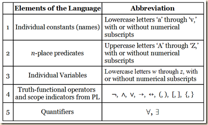
There are five elements in the language of predicate logic (RL).

1) Individual constants or names of specific items, and they are represented with lower case letters spanning from ‘a’ to ‘v’ (and expanded with subscript numerals).

2) n-place predicates, which predicate a constant or variable, or they relate constants or variables to one another. They are represented with capital letters from ‘A’ to ‘Z’ (and expanded with subscript numerals).

3) Individual variables, which can be substituted by certain constants, and they are represented with lowercase (often italicized) letters spanning from ‘w’ to ‘z’ (and expanded with subscript numerals).

4) Truth functional operators and scope indicators from the language of propositional logic (PL), namely, ¬, ∧, ∨, →, ↔, (, ), [, ], {, }.

5) Quantifiers, which indicate what portion of the set of items that can stand for a variable are to be taken into consideration in a part of a formulation. When indicating that the full portion is to be considered in some instance of a variable in a formula, we use the universal quantifier ∀. We can understand it to mean “all,” “every,” and “any.” But if we are to consider only a portion of the possible items that can substitute in for a variable, then we use the existential quantifier ∃, which can mean “some,” “at least one,” and the indefinite determiner “a.”

The purpose of the language of predicate logic is to express logical relations holding within propositions. There is the simple relation of predication to a subject, which would be a one-place predicate. There are also the relations of items within a predicate, as in “... is taller than ...”, which in this case is a two-place predicate, and so on. To say John is tall we might write Tj, and to write John is taller than Frank we could write Tjf. The number individuals that some predicate requires to make a proposition is called its adicity. And  when all the names have been removed from a predicational sentence, what remains is called an unsaturated predicate or a rheme. We might also formulate those above propositions using variables rather than constants, as in Tx and Txy. When dealing with variables, the domain of discourse D is the set of items that can be substituted for the variables in question, and this possible substitutions are called substitution instances for variables or just substitution instances. The domain is restricted if it contains only certain things and it is unrestricted if it includes all things. We may either explicitly stipulate what the domain is, which is common in formal logic, or the context of a discussion might implicitly determine the domain, and this domain can fluidly change as the discussion progresses. Also, in these cases with variables, we might further specify the quantities of the variables that we are to consider. So to say, everyone is taller than Frank we might write, (∀x)Txf. Someone is taller than Frank might be (∃x)Txf. Quantifiers have a scope in the formulation over which they apply. They operate just over the propositional contents to the immediate right of the quantifier or just over the complex propositional contents to the right of the parentheses.

 

 

Individual Constants (Names) and n-Place Predicates.

John is standing between Frank and Marry.

j = John

f = Frank

m = Mary

S = __ is standing between __ and __

Sjfm

 

Domain of Discourse, Individual Variables, and Quantifiers.

The domain of discourse D is all of the objects we want to talk about or to which we can refer.

D: positive integers

 

Individual variables are placeholders whose possible values are the individuals in the domain of discourse.

Bxyz = x is between y and z.

 

Universal quantifier: ∀. In English, “all,” “every,” and “any.”

(∀x)Mx

Everyone is mortal.

For every x, x is mortal.

All x’s are mortal.

For any x, x is mortal.

Every x is mortal.

 

Existential quantifier: ∃. In English, “some,” “at least one,” and the indefinite determiner “a.”

(∃x)Hx

Someone is happy.

For some x, x is happy.

Some x’s are happy.

For at least one x, x is happy.

There is an x that is happy.

 

Parentheses and Scope of Quantifiers

The ‘∀’ and ‘∃’ quantifiers operate over the propositional contents to the immediate right of the quantifier or over the complex propositional contents to the right of the parentheses. (Agler  254, quoting)

(∃x)Fx

[Above: ∃x ranges over Fx]

¬(∃x)(Fx∧Mx)

[Above: ¬(∃x) ranges over (Fx∧Mx)]

¬(∀x)Fx∧(∃y)Ry

[Above: ¬(∀x) ranges over Fx and (∃y) rangers over Ry]

(∃x)(∀y)(Rx↔My)

[Above: (∃x) ranges over (∀y)(Rx↔My) and (∀y) ranges over (Rx↔My)]

 

 

6.3 The Syntax of RL

 

In the language of predicate logic (RL), variables are either bound or free. They are bound if they fall under the scope of a quantifier that is quantifying specifically for that particular variable, and it is a free variable otherwise. An open sentence or an open formula is one with an n-place predicate P followed by n terms, where at least one of those variables is free. However, a closed sentence or a closed formula is one with an n-place predicate P followed by n terms, where none of those terms are free variables. The main operator in a well formed formula (wff) in RL is the one with the greatest scope, which means that the one that falls under no other operator’s scope is the main one. We consider the quantifiers as operators. Thus in (∃x)(Px∧Qx) the main operator is ∃x, because all the rest of the formula falls under the quantifier’s scope, and in ¬(∃x)(Px∧Qx) the main operator is the negation, because the quantifier falls under its scope, and the rest of the formula falls under the quantifier’s scope. And there are five rules that determine a wff in RL:  (i) An n-place predicate ‘P’ followed by n terms (names or variables) is a wff. (ii) If ‘P’ is a wff in RL, then ‘¬P’ is a wff. (iii) If ‘P’ and ‘Q’ are wffs in RL, then ‘P∧Q,’ ‘P∨Q,’ ‘P→Q,’ and ‘P↔Q’ are wffs. (iv) If ‘P’ is a wff in RL containing a name ‘a,’ and if ‘P(x/a)’ is what results from substituting the variable x for every occurrence of ‘a’ in ‘P,’ then ‘(∀x)P(x/a)’ and ‘(∃x)P(x/a)’ are wffs, provided ‘P(x/a)’ is not a wff. (v) Nothing else is a wff in RL except that which can be formed by repeated applications of (i) to (iv).

Free and Bound Variables

(∀x)(Fx→Bx)∨Wx

[Above: Wx does not fall under the scope of the quantifier and thus its variable is free.]

(∃z)(Pxy∧Wz)

[Above: only the z of Wz is bound.]

 

Main Operator in Predicate Wffs

[The main operator has the greatest scope.]

(∃x)(Px∧Qx)

[Above: (∃x) is the main operator.]

(∃x)(Px)∧(∃x)(Qx)

[Above: ∧ is the main operator.]

¬(∃x)(Px∧Qx)

[Above: ¬ is the main operator.]

(∀y)(∃x)(Rx→Py)

[Above: (∀y) is the main operator.]

 

The Formal Syntax of RL: Formation Rules.

Open formula: An open formula is a wff consisting of an n-place predicate ‘P’ followed by n terms, where one of those terms is a free variable.

Closed formula: A closed formula is a wff consisting of an n-place predicate ‘P’ followed by n terms, where every term is either a name or a bound variable.

 

Rule (iv): If ‘P’ is a wff in RL containing a name ‘a,’ and if ‘P(x/a)’ is what results from substituting the variable x for every occurrence of ‘a’ in ‘P,’ then ‘(∀x)P(x/a)’ and ‘(∃x)P(x/a)’ are wffs, provided ‘P(x/a)’ is not a wff.

Consider the wff:

Pb

Were we to say that we substitute every instance of the constant ‘b’ with the variable ‘x’, we would write:

P(x/b)

And we would obtain:

Px

It becomes a wff when we add a quantifier:

(∀x)Px

(∃x)Px

 

 

6.4 Predicate Semantics

 

In the language of predicate logic (RL) we will want to give interpretations for constants and for predicate formulations and also to give truth evaluations for well-formed formulas (wffs), including when they involve quantifiers. To do these things, we construct models, which specify the domain as well as the interpretation functions that assign objects in the domain to names, and n-tuples of objects to n-place predicates. On their basis, we valuate truth and falsity for formulas using a function that assigns T for when the named objects are among the tuples in the predicate’s interpretation, and F otherwise. When truth-evaluating quantified wffs in RL, we, intuitively speaking, give a universally quantified formula the value T if all substitutions for the variables make the formula true, and it is F otherwise; and for existentially quantified formulas, if there is at least one substitution that makes the formula true, it is evaluated as T, and F otherwise. For certain technical reasons, the actual procedure cannot involve substituting every possible name or object into the variables. We instead need to test for every object in the domain by thinking of each one being a potential interpretation for a constant, then seeing if these variant interpretations make the formula true or not. Despite the differences in notation, however, the more proper procedure conducts basically the same operation as the intuitive one. The evaluation rules for wffs in RL are the following:

1    v(Ra_i) = T if and only if the interpretation of ‘a_i’ is in ‘R.’

2    v(¬P) = T iff v(P) = F

v(¬P) = F iff v(P) = T

3    v(P∧Q) = T iff v(P) = T and v(Q) = T

v(P∧Q) = F iff v(P) = F or v(Q) = F

4    v(P∨Q) = T iff either v(P) = T or v(Q) = T

v(P∨Q) = F iff v(P) = F and v(Q) = F

5    v(P→Q) = T iff either v(P) = F or v(Q) = T

v(P→Q) = F iff v(P) = T and v(Q) = F

6    v(P↔Q) = T iff either v(P) = T and v(Q) = T or v(P) = F and v(Q) = F

v(P↔Q) = F iff either v(P) = T and v(Q) = F or v(P) = F and v(Q) = T

7    v(∀x)P = T iff for every name ‘a’ not in ‘P’ and every a-variant interpretation ‘P(a/x) = T.’

v(∀x)P = F iff for at least one ‘a’ not in ‘P’ and at least one a-variant interpretation ‘P(a/x) = F.’

8    v(∃x)P = T iff for at least one name ‘a’ not in ‘P’ and at least one a-variant interpretation ‘P(a/x) = T’.

v(∃x)P = F iff for every name ‘a’ not in ‘P’ and every a-variant interpretation ‘P(a/x) = F.

 

 

 

6.5 Translation from English to Predicate Logic

 

To translate between the language of predicate logic RL and colloquial English, we need to make a translation key to assign symbols to text, and we would follow the pattern given in this table:

 

 

6.6 Mixed and Overlapping Quantifiers

 

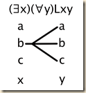
There is no simple and universally reliable procedure for translating all English sentences with quantifiers into the language of predicate logic (RL). Agler offers four steps that can help us make translations [quoting:] {1} Identify and symbolize any English expressions that represent quantifiers (and their bound variables) and propositional operators. {2} Translate any ordinary language predicates into predicates of RL. {3} Use the quantifiers from step 1 and the predicates from step 2 and represent the proposition that (1) expresses. {4} Read the predicate logic wff in English and check to see whether it captures the meaning of the sentence undergoing translation. When we have two quantifiers and they are both the same kind, their order will not matter. However, if one is universal and the other is existential, their order can change the meaning of the proposition. Here are four scenarios that illustrate:

(∀x)(∃y)Lxy     “Crush scenario”

Everyone loves someone.

[For any person, that person loves one (and/or another) person.]

(∃y)(∀x)Lxy     “Santa Claus scenario”

Someone is loved by everyone.

[There is one (and/or another) person who is loved by all other people.]

(∀y)(∃x)Lxy    “Stalker scenario”

Everyone is loved by someone.

[Each person is loved by at least one (and/or another) person.

(∃x)(∀y)Lxy   “Loving God scenario”

Someone loves everyone.

[One (and/or another) person loves every other person.]

 

 

Ch.7: Predicate Logic Trees

 

7.1 Four New Decomposition Rules

 

We can decompose quantified propositions of the language of predicate logic (RL) into logic trees, by using additional rules.

Negated Existential Decomposition (¬∃D)	Negated Universal Decomposition (¬∀D)
¬(∃x)P✔ (∀x)¬P	¬(∀x)P✔ (∃x)¬P

[Note that when the negation is moved, if there is a quantifier to the right, the negation is moved to the quantifier rather than jumping over to the proposition further to the right. So ¬(∃x)(∀y)Pxy becomes (∀x)¬(∀y)Pxy and not (∀x)(∀y)¬Pxy.]

Existential Decomposition (∃D)	Universal Decomposition (∀D)
(∃x)P✔ P(a/x)   where ‘a’ is an individual constant (name) that does not previously occur in the branch.	(∀x)P P(a/x)   where ‘a’ is any individual constant (name).

[Note that the universal quantifier is not checked, because for infinite domains, not all possible substitutions can be given in the tree.] The universal decomposition is further specified as:

Universal Decomposition (∀D)

(∀x)P P(a . . . v/x) Consistently replace every bound x with any individual constant (name) of your choosing (even if it already occurs in an open branch) under any (not necessarily both) open branch of your choosing.

 

Four kinds of decomposable propositions.

 

Four Decomposable Proposition Types

Existential                   (∃x)P

Universal                    (∀x)P

Negated existential      ¬(∃x)P

Negated universal        ¬(∀x)P

 

Negated Existential and Universal Decomposition.

Negated Existential Decomposition (¬∃D)	Negated Universal Decomposition (¬∀D)
¬(∃x)P✔ (∀x)¬P	¬(∀x)P✔ (∃x)¬P

 

1	¬(∃x)Px✔	P
2	¬(∀y)Wy✔	P
3	(∀x)¬Px	1¬∃D
4	(∃y)¬Wy	2¬∀D

 

Existential and Universal Decomposition.

Existential Decomposition (∃D)	Universal Decomposition (∀D)
(∃x)P✔ P(a/x)   where ‘a’ is an individual constant (name) that does not previously occur in the branch.	(∀x)P P(a/x)   where ‘a’ is any individual constant (name).

 

According to (∃D) and (∀D), an individual constant (name) is substituted for a bound variable in a quantified expression. This procedure is symbolized as ‘P(a/x)’ (i.e., replace x with ‘a’). Thus, if there is a quantified expression of the form ‘(∀x)P’ or ‘(∃x)P,’ a substitution instance of ‘P(a/x)’ replaces x’s bound by the quantifier with ‘a.’ (quoting Agler 286)

 

Universal Decomposition (∀D)

(∀x)P P(a . . . v/x) Consistently replace every bound x with any individual constant (name) of your choosing (even if it already occurs in an open branch) under any (not necessarily both) open branch of your choosing.

1	(∀x)(Px→Rx)	P
2	Pa∨Ra✔	P
3	/               \ Pa              Ra	2∨D
4	Pa→Ra         Pa→Ra	1∀D

 

Existential Decomposition (∃D)

(∃x)P✔ P(a/x)   where ‘a’ is an individual constant (name) that does not previously occur in the branch.

1	(∃x)Px✔	P
2	Pa	P
3	Pb	1∃D

 

 

 

7.2 Strategies for Decomposing Trees

 

To decompose propositions in the language of predicate logic (RL) the most efficiently in truth trees, we should follow these rules.

 

Strategic Rules for Decomposing Predicate Truth Trees

1. Use no more rules than needed.

2. Decompose negated quantified expressions and existentially quantified expressions first.

3. Use rules that close branches.

4. Use stacking rules before branching rules.

5. When decomposing universally quantified propositions, use constants that already occur in the branch.

6. Decompose more complex propositions before simpler propositions.

 

 

7.3 Logical Properties

 

Truth trees can determine logical properties of singular propositions, sets of propositions, and arguments in the language of predicate logic (RL). To test a proposition to see if it is a contradiction, we see if it makes a closed tree. If and only if it does is it a contradiction. To test a proposition to see if it is a tautology, we make a tree for its negation. If and only if it makes a closed tree is the original proposition a tautology. If it fails both these tests, it is a contingency. To check for the consistency of sets of propositions, we see if their tree has at least one open branch. If so, they are consistent. If instead the tree is closed, then they are inconsistent. To test for the validity of an argument, we negate the conclusion and make a tree for the full set of sentences. If they determine a closed tree, the original argument was valid. If it determines a tree with at least one completed open branch, it is invalid.

Completed open branch: A branch is a completed open branch if and only if (1) all complex propositions that can be decomposed into atomic propositions or negated atomic propositions are decomposed; (2) for all universally quantified propositions ‘(∀x)P’ occurring in the branch, there is a substitution instance ‘P(a/x)’ for each constant that occurs in that branch; and (3) the branch is not a closed branch.

1	(∀x)(¬Px→¬Rx)	P
2	(∀x)(Rx→Px)	P
3	¬Pa→¬Ra✔	1∀D
4	Ra→Pa✔ /                      \	2∀D
5	¬¬Pa                       ¬Ra                                /             \                /            \	3→D
6	¬Ra               Pa        ¬Ra             Pa                            O                  O            O              O	4→D

 

Closed tree: A tree is a closed tree if and only if all branches close.

Closed branch: A branch is a closed branch if and only if there is a proposition and its literal negation (e.g., ‘P’ and ‘¬P’). (quoting Agler 294)

1	(∀x)(Px→Qx)	P
2	(∃x)(Px∧¬Qx)✔	P
3	Pa→Qa✔	1∀D
4	Pb∧¬Qb✔	2∃D
5	Pb	4∧D
6	¬Qb /                  \ /                              \	4∧D
7	¬Pa                                    Qa	3→D
8	Pb→Qb                            Pb→Qb                         /                \                        /                \	1∀D
9	¬Pb              Qb                 ¬Pb              Qb                       X                 X                     X                  X	8→D

 

“Consistency: A set of propositions ‘{A, B, C, ..., Z}’ is consistent in RL if and only if there is at least one interpretation such that all of the propositions in the set are true.” (Agler 296)

to show that ‘{(∀x)Px, (∃x)Rx}’ is consistent in RL involves showing that there is at least one interpretation in a model where v(∀x)Px = T and v(∃x)Rx = T. Here is an example of such a model:

D = positive integers

P = {x | x is greater than 0}

R = {x | x is even}

(Agler 296)

“Thus, the presence of a completed open branch tells us that we can construct a model such that every proposition in the stack is true” (Agler 297).

[“Completed open branch: A branch is a completed open branch if and only if (1) all complex propositions that can be decomposed into atomic propositions or negated atomic propositions are decomposed; (2) for all universally quantified propositions ‘(∀x)P’ occurring in the branch, there is a substitution instance ‘P(a/x)’ for each constant that occurs in that branch; and (3) the branch is not a closed branch.”]

1	(∃x)Px	P
2	Pa	P
3	Pb O	1∃D

 

Inconsistency: A set of propositions ‘{P, Q, R, ..., Z}’ is shown by the truth-tree method to be inconsistent if and only if a tree of the stack of ‘P,’ ‘Q,’ ‘R,’ . . ., ‘Z’ is a closed tree; that is, all branches close.

(∀x)(Px→Rx), ¬(∀x)(¬Rx→¬Px)

1	(∀x)(Px→Rx)	P
2	¬(∀x)(¬Rx→¬Px)✔	P
3	(∃x)¬(¬Rx→¬Px)✔	2¬∀D
4	¬(¬Ra→¬Pa)	3∃D
5	Pa→Ra✔	1∀D
6	¬Ra	4¬→D
7	¬¬Pa✔	4¬→D
8	Pa /                  \	7¬¬D
9	¬Pa                    Ra   X                      X	5→D

 

“the truth-tree method can be used to determine whether a proposition ‘P’ is a tautology, contradiction, or contingency. In testing ‘P’ to see if it is a tautology, begin the tree with ‘¬P.’ If the tree closes, you know that it is a tautology. If the tree is open, then ‘P’ is either a contradiction or a contingency. Similarly, in testing ‘P’ to see if it is a contradiction, begin the tree with ‘P.’ If the tree closes, you know that it is a contradiction. If the tree is open, then ‘P’ is either a tautology or a contingency. Lastly, if the truth-tree test shows that ‘P’ is neither a contradiction nor a tautology, then ‘P’ is a contingency” (Agler 147).

(∃x)¬(∀y)[Px→(Qx∨¬Ry)]

[Below: There is at least one completed open branch, so it is not a contradiction.]

1	(∃x)¬(∀y)[Px→(Qx∨¬Ry)]✔	p
2	¬(∀y)[Pa→(Qa∨¬Ry)]✔	1∃D
3	(∃y)¬[Pa→(Qa∨¬Ry)]✔	2¬∀D
4	¬[Pa→(Qa∨¬Rb)]✔	3∃D
5	Pa	4¬→D
6	¬(Qa∨¬Rb)✔	4¬→D
7	¬Qa	6¬∨D
8	¬¬Rb	6¬∨D

[Below: Since the above tree is not closed, the original form is not a tautology. Since it is neither a contradiction nor a tautology, it is therefore a contingency.]

1	¬(∃x)¬(∀y)[Px→(Qx∨¬Ry)]✔	P
2	(∀x)¬¬(∀y)[Px→(Qx∨¬Ry)]✔	1¬∃D
3	¬¬(∀y)[Pa→(Qa∨¬Ry)]✔	2∀D
4	(∀y)[Pa→(Qa∨¬Ry)]	3¬¬D
5	Pa→(Qa∨¬Ra) /                                    \	4∀D
6	¬Pa                               Qa∨¬Ra✔                                O                              /                   \	5→D
7	Qa                 ¬Ra                                                               O                     O	6∨D

 

Equivalence: A pair of propositions ‘P’ and ‘Q’ is shown by the truth-tree method to be equivalent if and only if the tree of the stack of ‘¬(P↔Q)’ determines a closed tree; that is, all branches for ‘¬(P↔Q)’ close. 

(∀x)Px

¬(∃x)Px

[Below: The negated biconditional makes an open tree and thus they are not equivalent.]

1	¬[(∀x)Px↔¬(∃x)Px]✔ /                            \	P
2	(∀x)Px                ¬(∀x)Px	1¬↔D
3	¬¬(∃x)Px✔             ¬(∃x)Px	1¬↔D
4	(∃x)Px✔	3¬¬D
5	Pa	4∃D
6	Pa                           O	2∀D

 

(∀x)¬(Px∨Gx)

(∀y)(¬Py∧¬Gy)

[Below: Their negated biconditional makes a closed tree, and thus they are equivalent.]

1	¬{[(∀x)¬(Px∨Gx)]↔[(∀y)(¬Py∧¬Gy)]}✔ /                                                     \	P
2	(∀x)¬(Px∨Gx)                                ¬(∀x)¬(Px∨Gx)	1¬↔D
3	¬(∀y)(¬Px∧¬Gx)✔                         (∀y)(¬Px∧¬Gx)	1¬↔D
4	(∃y)¬(¬Px∧¬Gx)✔                                          |	3¬∀D
5	¬(¬Pa∧¬Ga)✔                                               |                     /              \                                                      |	4∃D
6	¬¬Pa✔    ¬¬Ga✔                                             |	5¬∧D
7	Pa                 Ga                                                  |	6¬¬D
8	¬(Pa∨Ga)✔  ¬(Pa∨Ga)✔                                    |	2∀D
9	¬Pa                 ¬Pa                                               |	8¬∨D
10	X                   ¬Ga                                               |                                           X                                                 |	8¬∨D
11	(∃x)¬¬(Px∨Gx)✔	2¬∀D
12	Pa∨Ga✔                                                                                         /                   \	11∃D
13	Pa                   Ga	12∨D
14	¬Pa∧¬Ga     ¬Pa∧¬Ga	3∀D
15	¬Pa               ¬Ga                                                                                    X                    X	14∧D

 

 

 

 

 

7.4 Undecidability and the Limits of the Predicate Tree Method

 

When we deal with the problem of universal instantiation causing us to repeat over and over a combination of existential and universal decomposition rules, we can instead apply the following new existential decomposition rule.

 

Unlike PL, RL is undecidable. That is, there is no mechanical procedure that can always, in a finite number of steps, deliver a yes or no answer to questions about | whether a given proposition, set of propositions, or argument has a property like consistency, tautology, validity, and the like. For some trees, the application of predicate decomposition rules will result in a process of decomposition that does not, in a finite number of steps, yield a closed tree or a completed open branch. (quoting Agler 317-318)

 

A use of (N∃D) requires that whenever we decompose an existentially quantified proposition ‘(∃x)P,’ we create a separate branch for any substitution instance for any substitution instance P(a₁/x), P(a₂/x), ..., P(a_n/x), already occurring in the branch containing ‘(∃x)P’ and branch a substitution instance ‘P(a_n+1/x)’ that is not occurring in that branch. (quoting Agler 318)

1	(∀x)(∃y)(Pxy)	P
2	(∃y)Pay✔ /                 \	1∀D
3	Paa                  Pab	2N∃D
4	O                 (∃y)Pby                                 /           |           \	1∀D
5	Pba        Pbb       Pbc                             O              O            .                                                               .                                                               .	4N∃D

 

 

 

Ch.8: Predicate Logic Derivations

 

8.1 Four Quantifier Rules

 

For the language of predicate logic (RL), there are four proof derivation rules to add to those of propositional logic (PL), namely:

Universal Elimination (∀E) From any universally quantified proposition ‘(∀x)P,’ we can derive a substitution instance ‘P(a/x)’ in which all bound variables are consistently replaced with any individual constant (name).

(∀x)P P(a/x)

∀E

 

Existential Introduction (∃Ι) From any possible substitution instance ‘P(a/x),’ an existentially quantified proposition ‘(∃x)P’ can be derived by consistently replacing at least one individual constant (name) with an existentially quantified variable.

P(a/x) (∃x)P

∃I

 

Universal Introduction (∀Ι) A universally quantified proposition ‘(∀x)P’ can be derived from a possible substitution instance ‘P(a/x)’ provided (1) ‘a’ does not occur as a premise or as an assumption in an open subproof, and (2) ‘a’ does not occur in ‘(∀x)P.’

P(a/x) (∀x)P

∀I

 

Existential Elimination (∃E) From an existentially quantified expression ‘(∃x)P,’ an expression ‘Q’ can be derived from the derivation of an assumed substitution instance ‘P(a/x)’ of ‘(∃x)P’ provided (1) the individuating constant ‘a’ does not occur in any premise or in an active proof (or subproof) prior to its arbitrary introduction in the assumption ‘P(a/x),’ and (2) the individuating constant ‘a’ does not occur in proposition ‘Q’ discharged from the subproof.

(∃x)P    | P(a/x)    | .    | .    | .    | Q Q

∃E

This new system of derivation is called RD. And corresponding to these are four additional strategic rules for making proofs in RL.

SQ#1(∀E): When using (∀E), the choice of substitution instances ‘P(a/x)’ should be guided by the individual constants (names) already occurring in the proof and any individual constants (names) occurring in the conclusion.
(Agler 328)

SQ#2(∃I): When using (∃I), aim at deriving a substitution instance ‘P(a/x)’ such that a use of (∃I) will result in the desired conclusion. (In other words, if the ultimate goal is to derive ‘(∃x)Px,’ aim to derive a substitution instance of ‘(∃x)Px,’ like ‘Pa,’ ‘Pb,’ ‘Pr,’ so that a use of (∃I) will result in ‘(∃x)Px.’)

SQ#3(∀I): When the goal proposition is a universally quantified proposition ‘(∀x)P,’ derive a substitution instance ‘P(a/x)’ such that a use of (∀I) will result in the desired conclusion.

SQ#4(∃E) Generally, when deciding upon a substitution instance ‘P(a/x)’ to assume for a use of (∃E), choose one that is foreign to the proof.

Universal Elimination (∀E).

Universal Elimination (∀E) From any universally quantified proposition ‘(∀x)P,’ we can derive a substitution instance ‘P(a/x)’ in which all bound variables are consistently replaced with any individual constant (name).

(∀x)P P(a/x)

∀E

1	(∀x)Px	P
2	Pa	1∀E

Existential Introduction (∃I)

Existential Introduction (∃Ι) From any possible substitution instance ‘P(a/x),’ an existentially quantified proposition ‘(∃x)P’ can be derived by consistently replacing at least one individual constant (name) with an existentially quantified variable.

P(a/x) (∃x)P

∃I

Zr ⊢ (∃x)Zx

1	Zr	P
2	(∃x)Zx	1∃I

Universal Introduction (∀I)

Universal Introduction (∀Ι) A universally quantified proposition ‘(∀x)P’ can be derived from a possible substitution instance ‘P(a/x)’ provided (1) ‘a’ does not occur as a premise or as an assumption in an open subproof, and (2) ‘a’ does not occur in ‘(∀x)P.’

P(a/x) (∀x)P

∀I

(∀x)Px ⊢ (∀y)Py

1	(∀x)Px	P
2	Pa	1∀E
3	(∀y)Py	2∀I

 

Existential Elimination (∃E)

Existential Elimination (∃E) From an existentially quantified expression ‘(∃x)P,’ an expression ‘Q’ can be derived from the derivation of an assumed substitution instance ‘P(a/x)’ of ‘(∃x)P’ provided (1) the individuating constant ‘a’ does not occur in any premise or in an active proof (or subproof) prior to its arbitrary introduction in the assumption ‘P(a/x),’ and (2) the individuating constant ‘a’ does not occur in proposition ‘Q’ discharged from the subproof.

(∃x)P    | P(a/x)    | .    | .    | .    | Q Q

∃E

1	(∃x)Px	P
2	| Pa	A/∃E
3	| (∃y)Py	2∃I
4	(∃y)Py	1,2–3∃E

 

8.2 Quantifier Negation (QN)

 

The four underived quantifier rules for making proofs in the language of predicate logic (RL) made a derivation system called RD. To this we add the derived equivalence rule quantifier negation (QN) to make the deduction system RD+. And since it is an equivalence rule, QN can apply to quantifiers that are not main operators.

Quantifier Negation (QN) From a negated universally quantified expression ‘¬(∀x)P,’ an existentially quantified expression ‘(∃x)¬P’ can be derived, and vice versa. Also, from a negated existentially quantified expression ‘¬(∃x)P,’ a universally quantified expression ‘(∀x)¬P’ can be inferred, and vice versa.

¬(∀x)P ⊣ ⊢ (∃x)¬P ¬(∃x)P ⊣ ⊢ (∀x)¬P

QN QN

1	¬(∀x)Px	P
2	(∃x)¬Px	1QN
3	¬(∀x)Px	2QN

 

1	¬(∃z)(Wzz∧Mz)	P
2	(∀z)¬(Wzz∧Mz)	1QN
3	¬(∃z)(Wzz∧Mz)	2QN

 

 

8.3 Sample Proofs

 

Agler illustrates the rules of the derivation system for making proofs in the language of predicate logic with a set of examples.

 

 

 

 

Agler, David. Symbolic Logic: Syntax, Semantics, and Proof. New York: Rowman & Littlefield, 2013.

 

 

 

 

.